Bessel Function of the Second Kind Y_v(x)

Quick answer

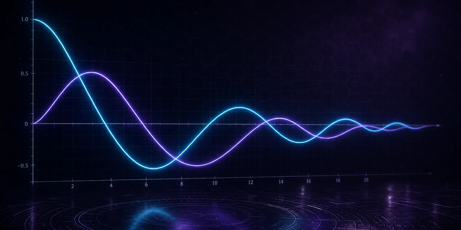
The Bessel function of the second kind Y_v(x) is the second independent solution to Bessel's equation on the positive real axis. It diverges at x = 0 and oscillates for large x with amplitude decay ~ 1/√x.

Introduction

Whenever a cylindrical region excludes the center, such as a coaxial line or an annulus, the general solution needs both J_v and Y_v. J_v alone cannot match every boundary if the inner radius is not zero. The Bessel Function Calculator helps you verify the J_v part while you study Y_v from references.

Start with J_v of the first kind if the bounded behavior at the origin is new to you. The introductory article explains the shared equation.

The home calculator emphasizes J_v for teaching stability; use this article to interpret Y_v from references and to know when it must appear in your sum.

For integer v, Y_v includes a logarithmic term near the origin mixed with J_v. That term is not a mistake; it is required by Frobenius theory when roots differ by an integer.

Radiation problems often package J_v and Y_v into Hankel functions H_v⁽¹⁾ = J_v + i Y_v and H_v⁽²⁾ = J_v − i Y_v with outgoing or incoming boundary conditions at infinity.

What does Y_v(x) represent physically?

Y_v models the radial factor that blows up toward the inner hole while still satisfying the outer boundary. It is the counterpart to cosine and sine pairs on an interval, but on a semi-infinite radial domain with a singularity at zero.

For integer v, Y_v includes a logarithmic term near the origin mixed with J_v. That term arises because two independent solutions cannot both be power-series regular at zero.

In radiation problems, Hankel functions H_v^(1,2) = J_v ± i Y_v package outgoing or incoming cylindrical waves.

On an annulus, coefficients A and B in A J_v + B Y_v are fixed by potentials or fields at inner and outer radii. The transcendental equation for allowed k couples both functions.

Numerical evaluation must start at x > 0. Plotting Y_v on the same axes as J_v away from zero shows comparable amplitudes even though their small-x behavior differs drastically.

Definitions and links to J_v

• Wronskian: J_v(x) Y_v'(x) − J_v'(x) Y_v(x) = 2/(π x)
• Recurrences mirror J_n with Y_n±1 terms
• H_v⁽¹⁾ = J_v + i Y_v, H_v⁽²⁾ = J_v − i Y_v

The Wronskian is a quick check when you have numerical J_v and Y_v from a library. It should match the stated factor up to roundoff.

Do not evaluate Y_v at x = 0 on a calculator expecting a finite number. Approach from above or work on an annulus r ∈ [r_in, r_out].

The Weber definition for integer n expresses Y_n through J_n and J_n ln x near zero. Reading that form once explains why log terms appear in coaxial homework.

Work with Y_v safely

1. Confirm the domain includes zero or not If the inner radius is zero and the solution must be finite, set the Y_v coefficient to zero and use only J_v.
2. Match boundary conditions on an annulus Solve linear equations for coefficients A and B in A J_v + B Y_v at r_in and r_out.
3. Evaluate away from the singularity Pick x ≥ r_in > 0. Compare J_v on the calculator with library Y_v at the same x.
4. Use Hankel functions for radiation Switch to H_v^(1,2) when imposing outgoing conditions at infinity in time-harmonic problems.

Example: why Y₀ matters on an annulus

On r ∈ [b, a] with fixed potentials at both radii, only J₀ is not enough because two constants of integration need two independent functions. A combination J₀(k r) + B Y₀(k r) can match both boundaries when k is chosen from a transcendental condition.

At x = 1, library values give Y₀(1) ≈ 0.0883 while J₀(1) ≈ 0.7652 from the calculator. The orders of magnitude differ but both are finite away from zero.

If you mistakenly use only J₀ on an annulus, you will find one free parameter too few to satisfy both boundaries unless the inner radius shrinks to zero.