
Quick answer
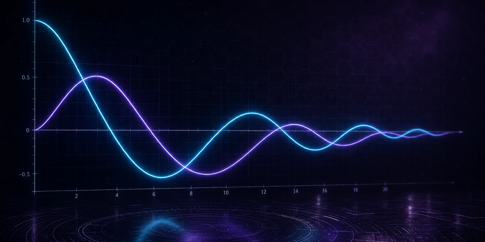
The Bessel function of the first kind Jv(x) is the regular solution at the origin to Bessel's equation. For integer v it oscillates and decays like a damped sine for large x.
Formula
- Bessel equation (cylindrical, order v):
- x2 y'' + x y′ + (x2 − v2) y = 0
- Regular solution at 0: y = Jv(x)
Introduction
If you work with circular waveguides, vibrating disks, or diffraction from round apertures, Jv(x) is already in your notes. The order v picks which radial mode you are in; the argument x is usually a scaled radius or frequency. Use the Bessel Function Calculator to turn each symbol into a number as you read.
Read what a Bessel function is for the big picture, and formulas for identities you will use daily.
Jv is the default solution when the origin is inside the domain and only finite amplitudes are physical. That single sentence eliminates Yv from many homework problems before you integrate anything.
Non-integer v appears in fractional-order waveguides and some fractional models. The calculator accepts fractional v; identities that assume integer factorials need extra care.
Large-x behavior is oscillatory with envelope decaying like 1/√x. That decay matters when you estimate how many modes contribute at the outer radius of a large disk.
What does Jv(x) represent?
Think of Jv(x) as the radial standing-wave shape that stays finite at the center of a disk. Higher v adds more nodes as you move outward.
For non-integer v the function is still defined, but some textbook identities that mix Jv±1 need care with analytic continuation.
Near x = 0, Jv(x) ~ (x/2)^v / Γ(v+1) for v ≥ 0, which shows how order controls steepness at the origin.
Orthogonality on [0, a] with weight x lets you expand initial data in sums of Jv at different zeros. That is the bridge from ODE homework to Fourier-Bessel series in PDE courses.
Hankel functions Hv(1,2) = Jv ± i Yv package outgoing and incoming cylindrical waves when time-harmonic radiation is modeled.
Useful identities (integer n)
- Jn−1(x) + Jn+1(x) = (2n/x) Jn(x)
- d/dx Jn(x) = (1/2)(Jn−1(x) − Jn+1(x))
- Orthogonality on [0,a] with weight x for mode sums
These recurrence relations explain why the calculator reports related orders alongside Jv(x) in real mode.
Sums of products of Jn at different zeros appear in series solutions for disks and cylinders.
The generating function e(x/2)(t − 1/t) expands in powers of t whose coefficients are Jn(x). It is a compact way to remember how orders couple.
How to check a value quickly
- Choose real mode Set x as a real number when your model uses a physical radius or frequency on the real line.
- Enter v and x Match the order in your boundary condition. Use the same scaling you used when deriving x.
- Read the table and plot Compare Jv(x) with your reference. Use the plot to see whether you are on an increasing or decreasing part of the curve.
- Verify one identity Pick a recurrence at your x if you have time. One identity check per session builds long-term confidence.
Example: J0(2) and J1(2)
With v = 0 and x = 2, J0(2) ≈ 0.2239. With v = 1, J1(2) ≈ 0.5767. The plot in real mode should show the first dip of J0 after x = 0 near that neighborhood, while J1 starts linearly small then grows.
Contrast mentally with Yv(x), which is singular at the origin but pairs with Jv in general solutions on annular domains.
Try v = 3 at x = 4 on the calculator: the value is smaller than J1(4) because higher orders emphasize larger radii in mode shapes.