Are Bessel functions the same as sine and cosine?

They play a similar role in circular geometry, but they solve a different equation with an x 2 term that couples amplitude and curvature. For large x, J v (x) looks like a damped oscillation, not a pure sinusoid.

What does the order v mean physically?

Often it counts angular nodes or selects a standing-wave mode. In quantum mechanics on a disk, v ties to angular momentum.

Where do I see Bessel functions in practice?

Waveguides, diffraction, vibrations, and heat flow on disks are common cases. The applications article at the end of this series lists several worked settings.

Can I use the site for complex arguments?

Yes. Switch to complex mode on the home calculator when z = x + i y is complex. Start with real mode until the geometry is clear.

What Is a Bessel Function? Definition and Uses

A clear starting point for Bessel functions: what they solve, how they behave, and how to try values on the Bessel Function Calculator or jump straight to the calculator section.

Open the calculator

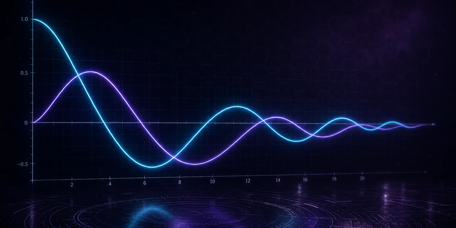
Quick answer

A Bessel function is a special function that solves Bessel's differential equation, which arises when you separate variables in cylindrical or circular geometry. The most common family is J_v(x), the Bessel function of the first kind of order v.

Formula

Bessel's equation (order v):
x² y^'' + x y^′ + (x² − v²) y = 0
Regular at x = 0: y = J_v(x)

Introduction

You meet Bessel functions whenever a physical setup has circular symmetry: a drumhead, a microwave mode in a round waveguide, light through a circular aperture, or heat in a disk. The radial part of the wave does not look like a plain sine; it looks like J_v(x) or a closely related cousin. The free Bessel Function Calculator on this site lets you evaluate those functions and plot them without installing software.

The label v is called the order. It counts how many nodes the radial pattern has near the center. The argument x is usually a dimensionless combination of radius and wavenumber, so the same symbol can mean different lengths in different problems. Keeping v and x straight is the first habit that prevents wrong mode numbers in homework and design notes.

This article is the first in a ten-part series on cylindrical Bessel functions. After you have the idea here, the formula guide collects the identities you will use daily, and the how to calculate Bessel functions article explains which numerical method fits each range of x.

You do not need heavy complex analysis to use Bessel functions well. You need a clear picture of what problem produced the equation, which solution stays finite at the center, and how to check one number before you trust a long derivation.

Students often confuse Bessel functions with trigonometric functions because both appear inside separated solutions. The difference is the extra x² term in the differential equation, which changes the spacing of zeros and the decay of peaks at large x.

What is a Bessel function, in plain terms?

Picture a vibrating circular membrane fixed at the edge. The motion separates into angular and radial parts. The radial factor must stay finite at the center and match zero at the rim. Those constraints pick Bessel functions as the natural shapes.

J_v(x) is the solution that stays bounded at x = 0 for real x. Another solution, Y_v(x), blows up at the origin and shows up when the center is excluded, such as around a hole or a line source. Modified versions I_v(x) and K_v(x) appear when hyperbolic growth or decay replaces oscillation.

Bessel functions are not polynomials. They are defined by series, integrals, or as solutions to the differential equation. Tables and software exist because closed forms in elementary functions are rare except for a few special orders.

In quantum mechanics on a disk, the angular momentum quantum number m appears in the angular factor e^{i m θ}, while the radial part is J_m(β r). In electromagnetics, the same J_n appears when you solve for the electric field inside a circular waveguide. The physics changes; the radial algebra repeats.

When two independent solutions are needed on an interval that includes the origin, you write a linear combination A J_v(x) + B Y_v(x). When the origin is part of the domain and only finite solutions are physical, B is often zero and J_v alone carries the mode.

The equation everything shares

x² y^'' + x y^′ + (x² − v²) y = 0
Two independent solutions for each order v
Bounded at 0 (real axis): J_v(x)

Every standard Bessel identity starts from this equation. Changing v changes the angular momentum in quantum problems and the mode index in waveguides. Changing the sign of the x² term leads to modified Bessel functions, which solve a related equation with exponential rather than oscillatory behavior.

For integer v, J_v(x) and J_-v(x) are related by a simple phase factor, which is why textbooks often focus on non-negative orders. The Wronskian of J_v and Y_v is proportional to 1/x, a fact you can use to verify numerical output from two libraries.

Series definitions express J_n(x) as a sum of powers of x/2 divided by factorials. That form is useful for small x and for understanding why J₀(0) = 1 while J_n(0) = 0 for n > 0.

Orthogonality relations on finite intervals let you expand piecewise profiles in sums of J_n at different zeros. That step is how boundary-value problems become countable mode sums in applied mathematics.

How to get from definition to a number

Name your order and argument Write down v from your boundary condition (mode number) and x from your scaled radius or frequency. Keep units consistent so x is dimensionless.
Pick the right family Use J_v for finite behavior at the origin, Y_v when the center is singular, and I_v or K_v for modified problems. If you are unsure which family your derivation produced, return to the differential equation sign.
Check one point on the calculator Open the calculator, enter v and x in real mode, and compare J_v(x) with your notes or a table.
Read the plot for context A single value is easy to mistype. The local curve shows whether you are near a zero, a peak, or an asymptotic tail.
Record your scaling Note whether x means k r, β a, or another product. Future you (and your grader) need the same convention.

Example: the lowest radial mode

For a disk of radius a with fixed rim, the lowest symmetric mode often involves J₀(k r) with J₀(k a) = 0 for some wavenumber k. The first zero of J₀ is about 2.4048, so k a ≈ 2.4048. That single transcendental condition fixes the smallest frequency at which the disk can resonate in this symmetric pattern.

Evaluating J₀(2) on the calculator gives roughly 0.2239, a moderate value on the way toward that first zero. At x = 2.4, J₀ is near zero, which matches the idea that you are close to the first root. Seeing both numbers anchors the abstract definition.

If you increase the order to v = 1 with the same x = 2, the value changes to about 0.5767 and the plot shows the curve starting from zero at the origin before rising. That contrast is how order v shapes real hardware and homework plots.

Frequently asked questions

Are Bessel functions the same as sine and cosine?: They play a similar role in circular geometry, but they solve a different equation with an x² term that couples amplitude and curvature. For large x, J_v(x) looks like a damped oscillation, not a pure sinusoid.
What does the order v mean physically?: Often it counts angular nodes or selects a standing-wave mode. In quantum mechanics on a disk, v ties to angular momentum.
Where do I see Bessel functions in practice?: Waveguides, diffraction, vibrations, and heat flow on disks are common cases. The applications article at the end of this series lists several worked settings.
Can I use the site for complex arguments?: Yes. Switch to complex mode on the home calculator when z = x + i y is complex. Start with real mode until the geometry is clear.

Start with one calculation

A Bessel function is the radial building block for circular problems, defined by Bessel's equation and labeled by order v. Knowing the definition is enough to read most engineering formulas; knowing one numeric check keeps you honest.

Use the series on this site in order, and keep the calculator open while you read.