
Quick answer
Bessel functions describe radial modes in cylindrical symmetry: electromagnetic fields in waveguides, vibrations of disks, quantum states on a disk, and diffraction from circular apertures all produce Jv, Yv, or modified forms.
Formula
- Waveguide: E_z ~ Jn(k_c r) with Jn(k_c a) = 0
- Disk vibration: w ~ Jn(α r) with Jn(α a) = 0
- Fraunhofer circular aperture: intensity ~ [2 J1(ka sin θ)/(ka sin θ)]2
Introduction
Physics textbooks scatter Bessel functions across chapters. The unifying idea is circular or cylindrical symmetry: when the Laplacian separates in polar coordinates, the radial factor is a Bessel function. The Bessel Function Calculator lets you evaluate that factor while you map each chapter to the same template.
If you need definitions or formulas first, read what is a Bessel function and worked examples. This closing article ties the series to labs and courses you may already be taking.
Electromagnetism, mechanics, quantum mechanics, and optics all reuse the same radial equation with different boundary words. Learning the template once saves rereading four separate derivations.
When a problem is not symmetric, Bessel functions may still appear after an integral transform or an approximation, but the cleanest examples stay on disks, cylinders, and circular apertures.
Carry one numeric habit through every chapter: pick v, pick x, calculate Jv, then ask whether the value matches the boundary story you told in words.
Where do physicists meet Bessel functions?
In electromagnetism, TE and TM modes in circular waveguides involve Jn and Yn on annular or solid conductors. Cutoff frequencies come from zeros of Jn.
In mechanics, the wave equation on a disk with fixed rim yields Bessel functions for radial displacement. The lowest symmetric mode uses J0 zeros.
In quantum mechanics, a particle on a disk has wavefunctions ψ ~ Jm(β r) ei m θ with β fixed by the boundary. The order m is angular momentum.
In optics, the Airy pattern from a circular aperture is built from J1 in the small-angle limit. Heat flow in steady cylindrical symmetry brings in modified functions Kv and Iv.
Plasma physics and acoustics add further examples, but the move is identical: separate variables, solve the radial ODE, apply boundaries, sum modes.
Representative setup equations
- Helmholtz in polar: (∇2 + k2) u = 0 → u ~ Jn(k r)
- Heat steady state: ∇2 T = 0 in cylinder → T ~ I0(κ r) or K0(κ r)
- Scattering phase: Hankel functions Hn(1,2) for outgoing waves
Each line is a template. Your parameters enter through boundary radii, permittivity, tension, or mass. The Bessel part is the same algebra with different symbols.
When outgoing radiation is required, replace pure Jn with Hankel functions, built from Jn and Yn as described in the second kind article.
Diffraction intensity patterns normalize by the on-axis value; the first zero of J1 sets the angular radius of the first dark ring in a circular aperture demo.
Map a physics problem to Jv
- Identify symmetry If the domain is circular or cylindrical, expect Bessel functions in the radial part.
- Separate variables Write u(r, θ, z) as products. Angular dependence gives ei m θ or sin(m θ), leaving Jm or Ym in r.
- Apply boundary conditions Zeros of Jm fix allowed k or β. Annular boundaries mix Jm and Ym.
- Evaluate amplitudes Use the calculator at interior points once modes are chosen.
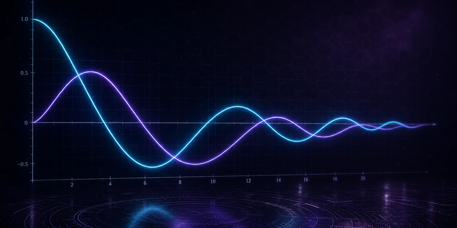
- Compare with graphs Visualize the radial factor with a plot so zeros line up with your geometric radii.
Example: circular aperture diffraction
On-axis intensity relative to the peak involves J1(x)/x with x = ka sin θ. At small angles, x is small and the ratio tends to 1/2 by series. At the first zero of J1, near x ≈ 3.8317, the pattern has a dark ring.
Plug x = 3.8 into the calculator for J1 to see a near-zero numerator, explaining the dark ring location in a demo lab.
Changing aperture radius a scales x at fixed angle, moving the ring positions. That scaling is easier to see numerically than to memorize multiple formulas.