Bessel Function Graphs: Zeros and Orders

Quick answer

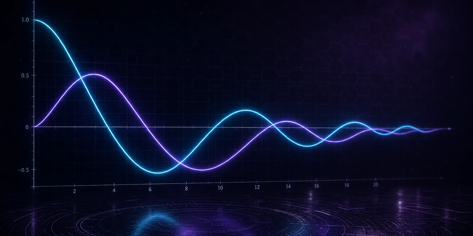
Graphs of J_v(x) show oscillation with decaying amplitude ~ 1/√x for large x, more zeros as v increases, and steeper rise near the origin for larger v. The calculator plot gives a local window around your chosen x.

Introduction

A table of values tells you one point; a graph tells you whether you picked a zero, a peak, or the wrong order entirely. Plotting is the fastest sanity check in cylindrical work, and the Bessel Function Calculator includes a local plot whenever you calculate.

Pair this page with worked examples and the calculator guide so you know how to regenerate figures and read every control.

Zeros of J_v are where mode conditions J_v(β a) = 0 lock allowed frequencies. A graph makes those crossings visible without solving transcendental equations by hand.

When you compare orders, overlay J₀ and J₁ on the same interval to see how extra nodes appear as v increases. That picture prevents confusing mode indices in multimode waveguides.

Modified functions should not be plotted on the same linear scale as J_v over large intervals because I_v grows exponentially. Use log scale or separate panels.

What should you look for on a graph?

Near the origin, J_v starts small for v > 0 and flat for v = 0. Count how many times the curve crosses zero before your boundary radius; that count informs mode labels.

Far to the right, peaks shrink and spacing approaches uniform, like a sine with slowly changing amplitude. Modified functions, by contrast, curve upward or downward without oscillation.

Complex arguments need separate real and imaginary plots or magnitude plots; start with real x until the picture is familiar.

The calculator embeds a window near your input x. Use it to see local curvature; export to a plotting tool when you need a full spectrum from 0 to 10a.

Derivative zeros correspond to turning points of the radial mode and link to J_v±1 through the derivative identity.

Graph features tied to formulas

• Zeros solve J_v(x) = 0
• Peaks satisfy local maxima of |J_v(x)|
• d/dx zeros link to J_v±1 via derivative identities

When a textbook says the first root of J₀, look near 2.4 on a J₀ plot. When it says the second, look near 5.5.

Superposing J₀ and J₁ on the same axes shows how order shifts phase and amplitude, useful in multimode waveguides.

Asymptotic envelopes √(2/(πx)) bound the oscillation at large x and explain why peaks shrink even as the function keeps crossing zero.

Build a useful graph

1. Fix v and scan x Hold order constant. Move x across your physical interval scaled to dimensionless variables.
2. Use the calculator local plot Enter a central x where you care. The embedded plot at the calculator shows nearby shape without exporting data.
3. Mark boundaries Draw vertical lines at scaled inner and outer radii. Intersections with zeros give mode conditions.
4. Compare orders Repeat for v and v+1 to see extra nodes.
5. Export for reports if needed For publication-quality figures, replot the same v and x range in your plotting tool using values checked on the calculator.

Example: reading J₀ from x = 0 to 8

J₀ crosses zero near 2.4, 5.5, and 8.7. Between zeros the curve alternates sign with decaying peaks. At x = 2 the calculator shows J₀(2) > 0 before the first crossing, so you know a disk mode with ka below 2.4 is not yet at the first root.

Overlaying J₁ on the same interval shows a first zero near 3.8, explaining why higher angular modes have different cutoff scales.

If your boundary is at x = 6 and you need the second zero of J₀, the graph shows you are past the first crossing near 2.4 but before the second near 5.5, which guides which mode index you are matching.