
Quick answer
The calculator evaluates Jv(x) in real mode and Jv(z) in complex mode, shows related orders, and plots the function near your input so you can verify textbook values quickly.
Formula
- Real mode: enter order v, real x
- Complex mode: enter v, real and imaginary parts of z
- Output: Jv, neighbors, and a local plot
Introduction
The Bessel Function Calculator on this site is built for learning and spot checks, not batch processing. It mirrors the formulas discussed in the blog so you can move from an equation to a number in seconds without leaving the topical map.
If you have not read the theory yet, start with what is a Bessel function. If you already know what to compute, see how to calculate Bessel functions for method background.
The calculator lives in the hero section of the home page with id calculator. Links that end in /#calculator scroll directly to the inputs, which is useful when you share homework links with classmates.
Real mode is the default for drumheads, waveguides, and any problem where the radial coordinate stays on the positive real axis. Complex mode appears when damping or phasor notation gives z a nonzero imaginary part.
After you click Calculate, read both the value table and the plot. The table answers what is Jv at this point; the plot answers whether that point sits on a rising branch, near a zero, or in the tail.
What the calculator shows
In real mode you get Jv(x) plus values that help with recurrence checks, such as neighbors in order when available. A plot centered near x shows local oscillation or decay.
In complex mode the tool reports real and imaginary parts, magnitude, and phase of Jv(z). That matters for damped waves where the argument is not purely real.
The interface stays on the home page so you can read articles in one tab and compute in another without losing context. Refreshing the page does not clear your last inputs if the browser restores form state.
Validation keeps v between −99 and 99 and x between −20 and 20 in real mode, which covers typical homework ranges. For extreme arguments, use a desktop library and treat the site as a sanity bracket.
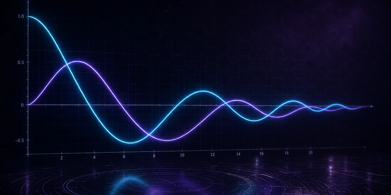
The graph draws Jv and Yv on x ∈ [0, 10] when you calculate in real mode, so you can compare families visually even though the primary output emphasizes Jv.
Inputs map to standard notation
- Order field → v in Jv
- Argument field → x or z
- Plot window → local behavior around your point
Match the v in your boundary condition, not an arbitrary index from a table unless you have converted units. Match the argument scaling used when you derived x from radius and wavenumber.
If a formula divides by x, avoid x = 0 unless you know the limit. The calculator will evaluate at small nonzero x if you need a hint for indeterminate forms.
Complex mode expects real and imaginary parts separately. That matches how most students write z = a + ib and reduces sign errors compared with typing a + ib as one opaque string.
When your course uses j for √−1 instead of i, the numeric value is the same; only the label on the imaginary box changes in your notes, not the mathematics.
Use the calculator in five steps
- Open the calculator section Go to calculator on the home page. The section scrolls into view from any blog article CTA.
- Choose real or complex mode Pick real mode for physical radii and frequencies on the real line. Pick complex mode when z has an imaginary part from damping or phasors.
- Enter order and argument Type v and x (or real and imaginary parts of z). Use the same numbers you would plug into a recurrence check from your formula sheet.
- Read the value table Compare Jv with your reference. Use neighbor values to verify identities without hand differentiation.
- Use the plot for sanity Confirm you are on the expected branch near a zero or peak. Change v slightly to see how the curve family shifts.
Example: checking J2(1.5) while reading
Set real mode, v = 2, x = 1.5. You should see J2(1.5) ≈ 0.1830. The plot shows a gentle rise from the origin before later oscillation sets in.
Change v to 0 with the same x to see how order reshapes the curve. That quick experiment is the same comparison used in worked examples later in the series.
Switch to complex mode with v = 2 and z = 3 + 5i to see a nontrivial imaginary part. Compare magnitude with your lecture notes if the course covers cylindrical functions in the complex plane.